Money Speed, or Velocity?
Your Money’s Rate of Change
In physics, speed is the measure of the rate of change of position of an object moving through space relative to some fixed point of observation. If you also reference a direction of travel, then one renames the observation “velocity.” The velocity of money measures how quickly money circulates in the direction of the economy — it reflects how actively money changes hands during a specific length of time. It is the number of times one dollar is spent to buy goods and services per unit of time. If the velocity of money is increasing, then more transactions are occurring between individuals in an economy. This indicator is used to monitor economic activity and assess the health of an economy. It can be written as:
Where gross domestic product is the total value in dollars of all final goods and services produced inside a country during a set period of time. If you add the term “nominal” before GDP, then you’re not counting the change of the value of the products or services you’re measuring during the length of time you’re measuring it. Generally, nominal is a sufficient characterization for usefulness without being super accurate.
Money Supply is given by M2 — a measure of all money circulating in an economy by cash, checking, savings deposits and money markets, of which we’ve written about before. More Money Chasing Fewer Stocks — July 1st, 2026
When consumers and businesses spend money more frequently buying and selling stuff, the velocity of money increases because GDP generally rises — the numerator in the equation. Conversely, when consumers and businesses reduce spending, the velocity of money falls for a fixed M2.
The Pandemic Plunge — and the Recovery
During the Covid pandemic, the Velocity of M2 Money Supply plunged to 1.104 by Q2 2020. Recently, it has been highlighted that the velocity of money has recovered from the pandemic low but it is still low compared to history. See the graph below where we plot the velocity of money from approximately 1960 to January of this year, as reported by the St. Louis Federal Reserve. The grey vertical bars represent recessions in the economy.
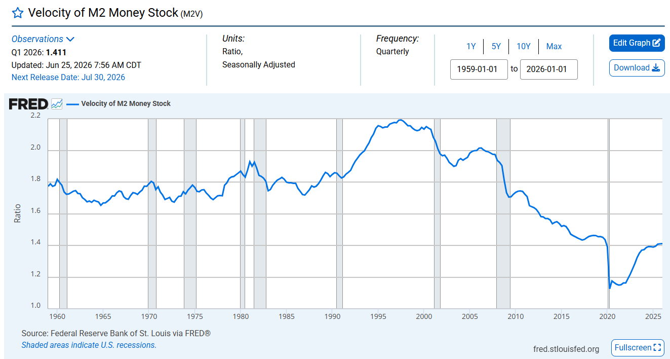
In this chart, we can see the velocity of money was falling after the 2008–09 Great Financial Crisis right up to the Covid era where it fell off a cliff. But since then, it has been increasing right up to the current time period. One can also notice a subtle trend: right before each recession the velocity of money is increasing, and then during and slightly after, the money velocity slows down. That makes economic sense, as less buying and selling of goods and services is concurrent with recessions so the velocity of money is obviously falling.
What Velocity Tells Us About Inflation
The velocity of money is also used to monitor “demand pull inflation.” This is an increase in prices of goods and services when demand outpaces supply. For example, if consumers receive income and spend it immediately, the same amount of money is used repeatedly for transactions at a faster turnover, increasing demand for goods and services while the money supply AND the supply of goods and services are both constant. This puts upward pressure on prices leading to inflation. This occurred strongly during the Covid era — demand went through the roof with supply constrained and prices rose accordingly as buyers hit Amazon like a tsunami, while simultaneously the government was printing money with the surge!
On the other hand, when the velocity of money falls, spending declines and inflation pressure falls, leading to lowering inflation often concurrent with recessions. The velocity of money therefore is a competing measure between changes in M2 and changes in GDP, and we can summarize it as follows:
What This Means for the Market — and BlueFire
From the graph, we would conclude that the falling velocity of money is not a concern at this point. Low velocity means money is sitting idle in savings rather than moving through the economy. The indicator is low but the economy is still growing generally — GDP is positive and M2 isn’t stationary but still increasing. Their ratio is stabilizing, which is not bad for the stock market. It portends the equity market returning to stock-specific fundamentals as their main driver. Only time will tell for sure, however.

Investments involve risk and, unless otherwise stated, are not guaranteed. Information provided is for educational purposes only. Be sure to first consult with a qualified financial adviser and/or tax professional before implementing any strategy discussed herein. Past performance is not indicative of future performance.